

Cluster analysis
A cluster is a collection of data objects that are similar to one another within the same cluster and are dissimilar to the objects in other clusters. The process of grouping a set of physical or abstract objects into classes of similar objects is called clustering.
Clustering techniques apply when there is no class to be predicted but rather when the instances are to be divided into natural groups. These clusters presumably reflect some mechanism at work in the domain from which instances are drawn, a mechanism that causes some instances to bear a stronger resemblance to each other than they do to the remaining instances. Clustering naturally requires different techniques to the classification and association learning.
Clustering differs from classification in that there is no target variable for clustering. The clustering task does not try to classify, estimate, or predict the value of a target variable. Instead, clustering algorithms seek to segment the entire data set into relatively homogeneous subgroups or clusters, where the similarity of the records within the cluster is maximized, and the similarity to records outside this cluster is minimized. By definition this is an example of unsupervised learning.
Applications
Business: Businesses collect large amounts of information on current and potential customers. Clustering can be used to segment customers into small number of groups for additional analysis and marketing activities
Information Retrieval: The World Wide Web consists of billions of Web pages, and the results of a query to a search engine can return thousands of pages. Clustering can be used to group these search results into a small number of clusters, each of which captures a particular aspect of the query. For instance, a query of “movie” might return Web pages grouped into categories such as reviews, trailers, stars, and theaters. Each category (cluster) can be broken into subcategories (subclusters), producing a hierarchical structure that further assists a user’s exploration of the query results.
Climate: Understanding the Earth’s climate requires finding patterns in the atmosphere and ocean. Cluster analysis has been applied to find patterns in the atmospheric pressure of polar region and areas of the ocean that have significant impact on land climate.
Biology: used to derive plant and animal taxonomies, categorize genes with similar functionality, and gain insight into structures inherent in populations.
Types of clustering algorithm
In general, the major clustering methods can be classified into the following categories.
1. Partitioning methods
Given a database of n objects or data tuples, a partitioning method constructs k partitions of the data, where each partition represents a cluster and k ≤ n. Given the number of partitions (k) to construct, a partitioning method creates an initial partitioning. It then uses an iterative relocation technique that attempts to improve the partitioning by moving objects from one group to another. The algorithms that use such methods are k-means algorithm, k-medoids algorithm etc.
2. Hierarchical Methods
A hierarchical method creates a hierarchical decomposition of the given set of data objects. If we permit clusters to have subclusters, then we obtain a hierarchical clustering, which is a set of nested clusters that are organized as a tree. Each node (cluster) in the tree (except for the leaf nodes) is the union of its children (subclusters), and the root of the tree is the cluster containing all the objects. A hierarchical method can be classified as being either agglomerative or divisive, based on how the hierarchical decomposition is formed.
Hierarchical methods suffer from the fact that once a step (merge or split) is done, it can never be undone. This rigidity is useful in that it leads to smaller computation costs by not having to worry about a combinatorial number of different choices. However, such techniques cannot correct erroneous decisions.
3. Density based methods
Most partitioning methods cluster objects based on the distance between objects. Such methods can find only spherical-shaped clusters and encounter difficulty at discovering clusters of arbitrary shapes. Other clustering methods have been developed based on the notion of density. Their general idea is to continue growing the given cluster as long as the density (number of objects or data points) in the “neighborhood” exceeds some threshold; that is, for each data point within a given cluster, the neighborhood of a given radius has to contain at least a minimum number of points. Such a method can be used to filter out noise (outliers) and discover clusters of arbitrary shape. DBSCAN and its extension, OPTICS, are typical density-based methods that grow clusters according to a density-based connectivity analysis.
4. Grid-based methods
Grid-based methods quantize the object space into a finite number of cells that form a grid structure. All of the clustering operations are performed on the grid structure (i.e., on the quantized space). The main advantage of this approach is its fast processing time, which is typically independent of the number of data objects and dependent only on the number of cells in each dimension in the quantized space.
5. Model-based methods:
Model-based methods hypothesize a model for each of the clusters and find the best fit of the data to the given model. A model-based algorithm may locate clusters by constructing a density function that reflects the spatial distribution of the data points. It also leads to a way of automatically determining the number of clusters based on standard statistics, taking “noise” or outliers into account and thus yielding robust clustering methods.
Only the first three methods are of interest to us.
Partitioning algorithm
Partitioning algorithm divides the data into k groups, which together satisfy the following requirements:
- Each group must contain at least one object, and
- Each object must belong to exactly one group.
These heuristic clustering methods work well for finding spherical-shaped clusters in small to medium-sized databases. The clusters are formed to optimize an objective partitioning criterion, such as a dissimilarity function based on distance, so that the objects within a cluster are “similar,” whereas the objects of different clusters are “dissimilar” in terms of the data set attributes.
K-means Clustering algorithm
K-means defines a cluster in terms of a centroid, which is usually the mean of a group of points. We first choose K initial centroids, where K is a user specified parameter, namely, the number of clusters desired. Each point is then assigned to the closest centroid, and each collection of points assigned to a centroid is a cluster. The centroid of each cluster is then updated based on the points assigned to the cluster. We repeat the assignment and update steps until no point changes clusters, or equivalently, until the centroids remain the same.
K-means is formally described by following algorithm:
Algorithm
Input:
k: the number of clusters,
D: a data set containing n objects.
Output: A set of k clusters.
Method:
1. Arbitrarily choose k objects from D as the initial cluster centers;
2. Repeat
2.1 Form k clusters by assigning each point to its closest centroid.
2.2 Recompute the centroid of each cluster.
3. Until Centroids do not change
The operation of K-means is illustrated in Figure 1, which shows how, starting from three centroids, the final clusters are found in three assignment-update steps. These figure shows the centroids at the start of the iteration and the assignment of the points to those centroids. The centroids are indicated by the “+” symbol; all points belonging to the same cluster have the same outlines encircled by dotted curves. In the first step, shown in Figure 1(a), points are assigned to the initial centroids (chosen randomly), which are all in the larger group of points. For this
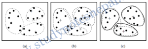
example, we use the mean as the centroid. After points are assigned to a centroid, the centroid is then updated. In the second step, points are assigned to the updated centroids, and the centroids are updated again which are shown in Figures 1(b) and 1(c). When the K-means algorithm terminates in Figure 1(c), because no more changes occur, the centroids have identified the natural groupings of points
Example 1.
D={2, 3, 4, 10, 11, 12, 20, 25, 30}
Divide into three clusters
—Refer class notes—
Example 2.
Generate cluster from following data set using K-means algorithm (take k= 2 and consider up to 2 iterations)
T1: Bread, Jelly, Butter
T2: Bread, Butter
T3: Bread, Milk, Butter
T4: Coke, Bread
T5: Coke, Milk
— Refer Class Notes—
Strength
K-means is simple and can be used for a wide variety of data types. It works well when the clusters are compact clouds that are rather well separated from one another. The method is relatively scalable and efficient in processing large data sets, even though multiple runs are often performed.
Weakness
K-means also has trouble clustering data that contains outliers. Outlier detection and removal can help significantly in such situations. The k-means method is not suitable for discovering clusters with nonconvex shapes or clusters of very different size. Finally, K-means is restricted to data for which there is a notion of a center (centroid) so it might not be applicable in some applications, such as when data with categorical attributes are involved.
Hierarchical Clustering
Hierarchical clustering techniques are a second important category of clustering methods. As with K-means, these approaches are relatively old compared to many clustering algorithms, but they still enjoy widespread use.
A hierarchical clustering method works by grouping data objects into a tree of clusters. Hierarchical clustering methods can be further classified as either agglomerative or divisive, depending on whether the hierarchical decomposition is formed in a bottom-up (merging) or top down (splitting) fashion. The quality of a pure hierarchical clustering method suffers from its inability to perform adjustment once a merge or split decision has been executed. That is, if a particular merge or split decision later turns out to have been a poor choice, the method cannot backtrack and correct it.
In general, there are two types of hierarchical clustering methods:
Agglomerative: Start with the points as individual clusters and, at each step, merge the closest pair of clusters. This requires defining a notion of cluster proximity.
Divisive: Start with one, all-inclusive cluster and, at each step, split a cluster until only singleton clusters of individual points remain. In this case, we need to decide which cluster to split at each step and how to do the splitting.
A hierarchical clustering is often displayed graphically using a tree-like diagram called a dendrogram, which displays both the cluster-subcluster relationships and the order in which the clusters were merged (agglomerative view) or split (divisive view).
Agglomerative Clustering
Many agglomerative hierarchical clustering techniques are variations on a single approach: starting with individual points as clusters, successively merge the two closest clusters until only one cluster remains. In general, agglomerative algorithms are more frequently used in real world applications than divisible methods.
Algorithm
1. Compute the proximity matrix, if necessary.
2. Repeat
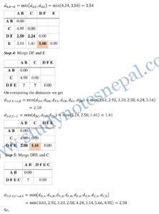
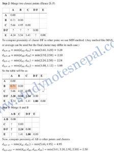
2.1. Merge the closest two clusters.
2.2. Update the proximity matrix to reflect the proximity between the new cluster and the
original clusters.
3. Until Only one cluster remains.
Defining inter-cluster similarity

The key operation of Algorithm for agglomerative clustering is the computation of the proximity (distance) between two clusters. For example, many agglomerative hierarchical clustering techniques, such as MIN, MAX, and Group Average, come from a graph-based view of clusters. MIN defines cluster proximity as the proximity between the closest two points that are in different clusters, or using graph terms, the shortest edge between two nodes in different subsets of nodes. Alternatively, MAX takes the proximity between the farthest two points in different clusters to be the cluster proximity, or using graph terms, the longest edge between two nodes in different subsets of nodes. The group average technique, defines cluster proximity to be the average pairwise proximities (average length of edges) of all pairs of points from different clusters.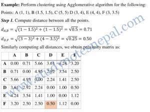
Divisive Method
A divisive algorithm starts from the entire set of samples X and divides it into a partition of subsets, then divides each subset into smaller sets, and so on until each object forms a cluster on its own or until it satisfies certain termination conditions, such as a desired number of clusters is obtained or the diameter of each cluster is within a certain threshold.. Thus, a divisive algorithm generates a sequence of partitions that is ordered from a coarser one to a finer one. In this case, we need to decide which cluster to split at each step and how to do the splitting. For a large data set, this method is computationally expensive.
Strength
Such algorithms are typically useful for the application such as creation of a taxonomy which requires a hierarchy of clusters. Also, there have been some studies that suggest that these algorithms can produce better-quality clusters.
Weakness
Agglomerative hierarchical clustering algorithms are expensive in terms of their computational and storage requirements. The hierarchical clustering method, though simple, often encounters difficulties regarding the selection of merge or split points. The fact that all merges are final can also cause trouble for noisy, high-dimensional data, such as document data
Density based clustering
To discover clusters with arbitrary shape, density-based clustering methods have been developed. These typically regard clusters as dense regions of objects in the data space that are separated by regions of low density (representing noise). DBSCAN grows clusters according to a density-based connectivity analysis. Density-based clustering locates regions of high density that are separated from one another by regions of low density. DBSCAN is a simple and effective density-based clustering algorithm that illustrates a number of important concepts that are important for any density-based clustering approach.
DBSCAN: Density-Based Spatial Clustering of Applications with Noise
DBSCAN algorithm grows regions with sufficiently high density into clusters and discovers clusters of arbitrary shape in spatial databases with noise. It defines a cluster as a maximal set of density-connected points.
In the center-based approach, density is estimated for a particular point in the data set by counting the number of points within a specified radius (Eps or ɛ) of that point. This includes the point itself. The size of epsilon neighborhood (ε) and the minimum points in a cluster (m) are user defined parameters.
The basic ideas of density-based clustering involve a number of new definitions.
Core points:
These points are in the interior of a density-based cluster. A point is a core point if the number of points within a given neighborhood around the point as determined by the distance function and a user specified distance Eps (or ɛ), exceeds a certain threshold, MinPts. In figure 3, if we suppose minpts=7, A is a core point because its neighborhood contains seven points (including itself).
Border points:
A border point is not a core point, but falls within the neighborhood of a core point. In figure 3, B is a border point because its neighborhood doesn’t satisfy minpts threshold but contains points which are within neighborhood of another core point i.e. A.
Noise points:
noise point is any point that is neither a core point nor a border point. In figure 3, C is a noise point because it is neither core nor border point.

Directly density reachable points:
Given a set of objects, D, we say that an object p is directly density-reachable from object q if p is within the ɛ-neighborhood of q, and q is a core object.
Density reachable points
An object p is density-reachable from object q with respect to ɛ and MinPts in a set of objects, D, if there is a chain of objects p1, . . . , pn, where p1 = q and pn = p such that pi+1 is directly density reachable from pi with respect to ɛ and MinPts.
Density connected points
An object p is density-connected to object q with respect to ɛ and MinPts in a set of objects, D, if there is an object such that both p and q are density-reachable from o with respect to ɛ and MinPts.
For example:

Consider Figure 4 for a given ɛ represented by the radius of the circles. let MinPts = 3. Based on the above definitions:
Of the labeled points, m, p, o and r are core objects because each is in a ɛ-neighborhood containing at least three points.
q is directly density-reachable from m and m is directly density-reachable from p
q is density-reachable from p because q is directly density-reachable from m and m is directly density-reachable from p. However, p is not density-reachable from q because q is not a core object. Similarly, r and s are density-reachable from o, and o is density-reachable from r.
o, r, and s are all density-connected.
Algorithm
- Label all points as core, border, or noise points.
- Eliminate noise points,
- Put an edge between all core points that are within Eps (or ɛ) of each other.
- Make each group of connected core points into a separate cluster.
- Assign each border point to one of the clusters of its associated core points.
Strength
Because DBSCAN uses a density-based definition of a cluster, it is relatively resistant to noise and can handle clusters of arbitrary shapes and sizes. Thus, DBSCAN can find many clusters that could not be found using K-means.
Weakness
DBSCAN has trouble when the clusters have widely varying densities. It also has trouble with high-dimensional data because density is more difficult to define for such data.
References
[1] J. Han and K. Micheline, Data Mining: Concepts and Techniques, San Francisco: Elsevier Inc., 2006.
[2] P.N. Tan, M. Steinbach and V. Kumar, INTRODUCTION TO DATA MINING, New York: PEARSON Addison Wesley, 2006.
[3] D. T. LAROSE, DISCOVERING KNOWLEDGE IN DATA An Introduction to Data Mining, New Jersey: John Wiley & Sons, Inc., 2005.