

Introduction
Many business enterprises accumulate large quantities of data from their day-to-day operations. For example, huge amounts of customer purchase data are collected daily at the checkout counters of grocery stores. Table 1 illustrates an example of such data, commonly known as market basket transactions. Each row in this table corresponds to a transaction, which contains a unique identifier labeled TID and a set of items bought by a given customer. Retailers are interested in analyzing the data to learn about the purchasing behavior of their customers. Such valuable information can be used to support a variety of business-related applications such as marketing promotions, inventory management, and customer relationship management.

Association analysis is a methodology which is useful for discovering interesting relationships hidden in large data sets. The uncovered relationships can be represented in the form of association rules or sets of frequent items. For example, the following rule can be extracted from the data set shown in Table 1:
{Diapers} → {Beer}
The rule suggests that a strong relationship exists between the sale of diapers and beer because many customers who buy diapers also buy beer. Retailers can use this type of rules to help them identify new opportunities for cross-selling their products to the customers.
Association rules take the form “If antecedent, then consequent,” along with a measure of the support and confidence associated with the rule. Typically, association rules are considered interesting if they satisfy both a minimum support threshold and a minimum confidence threshold. Such thresholds can be set by users or domain experts. For example, a particular supermarket may find that of the 1000 customers shopping on a Thursday night, 200 bought diapers, and of the 200 who bought diapers, 50 bought beer. Thus, the association rule would be: “If buy diapers, then buy beer,” with a support of 50/1000 = 5% and a confidence of 50/200 = 25%.
If the items or attributes in an association rule reference only one dimension, then it is a single-dimensional association rule. For example:
buys(X, “computer”) → buys(X, “antivirus software”)
If a rule references two or more dimensions, such as the dimensions age, income, and buys, then it is a multidimensional association rule. The following rule is an example of a multidimensional rule:
age(X, “30. . . 39”) ∧ income(X, “42K . . . 48K”) → buys(X, “high resolution TV”)
Examples of association tasks in business and research include:
- Investigating the proportion of subscribers to your company’s cell phone plan that respond positively to an offer of a service upgrade
- Examining the proportion of children whose parents read to them who are themselves good
readers - Predicting degradation in telecommunications networks
- Finding out which items in a supermarket are purchased together, and which items are never purchased together
- Determining the proportion of cases in which a new drug will exhibit dangerous side effects
The basic ideas of Association rule mining involve a number of new definitions
Itemsets
Let I = {I1, I2. . . I3} be a set of items. An itemset is a set of items contained in I, and a k-itemset is an itemset containing k items. In other words, itemset is collection of zero or more items. For example, {Bread, Milk} is a 2-itemset, and {Bread, Milk, Cola} is a 3-itemset, each from the Item set in table 1.
Support count
Support count for an itemset is the number of transaction or market basket containing all items in the itemset l.
Support
The supports for a particular association rule A → B is the proportion of transactions in D that contain both A and B. That is,
![]()
Support of a rule determines how often a rule is applicable to a given data set.
Confidence
The confidence c of the association rule A → B is a measure of the accuracy of the rule, as determined by the percentage of transactions in D containing A that also contains B. In other words,
![]()
Confidence determines how frequently items in B appear in the transactions that contain A.
Consider the rule {Milk, Diapers} → {beer}. Since the support count for {Milk, Diapers, Beer} is 2 and the total number of transactions is 5, so the rule’s support is 2/5 = 0.4. The rule’s confidence is obtained by dividing the support count for {Milk, Diapers, Beer} i.e. items in both antecedent and consequent (or A∪B in the rule A→B) by the support count for {Milk, Diapers} i.e. items in only antecedent (or A in the rule A→B). Since there are 3 transactions that contain both milk and diapers, the confidence for this rule is 2/3 = 0.67
Association Rule Discovery
Given a set of transactions T, find all the rules having support ≥ minsup and confidence ≥ minconf, where minsup and minconf are the corresponding support and confidence thresholds.
Some of approaches for association rules mining are:
Brute- Force Approach
A brute-force approach for mining association rules is to compute the support and confidence for every possible rule. This approach is prohibitively expensive because there are exponentially many rules that can be extracted from a data set. More specifically, the total number of possible rules extracted from a data set that contains d items is
R=3d-2d+r + 1
Even for the small data set shown in Table 6.1, this approach requires us to compute the support and confidence for 36– 27+ 1 = 602 rules. More than 80% of the rules are discarded after applying minsup = 20% and minconf = 50%, thus making most of the computations become wasted.
Mining association rules
A common strategy adopted by many association rule mining algorithms is to decompose the problem into two major subtasks:
- Frequent Itemset Generation, whose objective is to find all the itemsets that satisfy the minsup threshold. These itemsets are called frequent itemsets.
- Rule Generation, whose objective is to extract all the high-confidence rules from the frequent itemsets found in the previous step. These rules are called strong rules.
Itemset Lattice
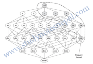
A lattice structure can be used to enumerate the list of all possible itemsets. Figure 1 shows an itemset lattice for {a, b, c, d, e}. In general, a data set that contains k items can potentially generate up to 2k – 1 frequent itemsets, excluding the null set. Because k can be very large in many practical applications, the search space of itemsets that need to be explored is exponentially large.
Apriori Principle
If an itemset is frequent, then all of its subsets must also be frequent.
Suppose {c, d, e} is a frequent itemset. Clearly, any transaction that contains {c, d, e} must also contain its subsets, {c, d}, {c, e}, {d, e}, {c}, {d}, and {e}. As a result, if {c, d, e} is frequent, then all subsets of {c, d, e} (i.e., the shaded itemsets in figure 1) must also be frequent.
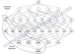
Conversely, if an itemset such as {a, b} is infrequent, then all of its supersets must be infrequent too. As illustrated in Figure 2, the entire subgraph containing the supersets of {a, b} can be pruned immediately once {a, b} is found to be infrequent. This strategy of trimming the exponential search space based on the support measure is known as support-based pruning. Such a pruning strategy is made possible by a key property of the support measure, namely, that the support for an itemset never exceeds the support for its subsets. This property is also known as the anti-monotone property of the support measure.
Apriori Algorithm
1. Let k=1
2. Generate frequent itemsets of length 1
3. Repeat until no new frequent itemsets are identified
3.1 Generate length (k+1) candidate itemsets from length k frequent itemsets
3.2 Prune candidate itemsets containing subsets of length k that are infrequent
3.3 Count the support of each candidate by scanning the DB
3.4 Eliminate (prune) candidates that are infrequent, leaving only those that are frequent.
Example of apriori algorithm
For the transaction database, D of following table, we use apriori algorithm to compute frequent
itemset. We suppose minsup count=2.
— Refer class notes—
Generating association rules from frequent itemsets
Once the frequent itemsets from transactions in a database D have been found, it is straightforward to generate strong association rules from them (where strong association rules satisfy both minimum support and minimum confidence).
For each frequent itemset l, generate all nonempty subsets of l.
For every nonempty subset s of l, output the rule “s → (l – s) if support count(l)/support count(s) ≥ min_conf, where min_conf is the minimum confidence threshold.
Because the rules are generated from frequent itemsets, each one automatically satisfies minimum support threshold.
Example
From apriori method we have computed many frequent itemsets. One of them is I= {A, B, E}. The nonempty subsets of I are {A}, {B}, {E}, {A, B}, {A, E} and {B, E}. The association rules that can be generated are as follows:
{A} → {B, E} confidence = 2/6 = 33%
{B} → {A, E} confidence = 2/7 = 29%
{E} → {A, B} confidence = 2/2 = 100%
{A, B} → {E} confidence = 2/4 = 50%
{A, E} → {B} confidence = 2/2 = 100%
{B, E} → {A} confidence = 2/2 = 100%
So, if we suppose the minimum confidence to be 70%, only {E} → {A, B}, {A, E} → {B}, {B, E} → {A} are strong association rules.
Remember that association rules can be derived from each of 2-frequent itemset, 3-frequent itemset and so on.
FP growth
FP-growth algorithm takes a radically different approach to discovering frequent itemsets than apriori algorithm. The algorithm does not follow the generate-and-test paradigm of Apriori. Instead, it encodes the data set using a compact data structure called an FP-tree and extracts frequent itemsets directly from this structure.
FP-growth adopts a divide-and-conquer strategy. First, it compresses the database representing frequent items into a frequent-pattern tree, or FP-tree, which retains the itemset association information. It then divides the compressed database into a set of conditional databases (a special kind of projected database), each associated with one frequent item or “pattern fragment,” and mines each such database separately.
For Example
Construction of FP Tree for the transactions of Table 2:
The first scan of the database is the same as Apriori, which derives the set of frequent items (1 itemsets) and their support counts (frequencies).
Let the minimum support count be 2.
The set of frequent items is sorted in the order of descending support count. This resulting set or list is denoted L. Thus, we have L= {{B: 7}, {A: 6}, {C: 6}, {D: 2}, {E: 2}}.
An FP-tree is then constructed as follows. First, create the root of the tree, labeled with “null.” Scan database D a second time. The items in each transaction are processed in L order (i.e., sorted according to descending support count), and a branch is created for each transaction. For example, the scan of the first transaction, “T1: A, B, E,” which contains three items (B, A, E in L order), leads to the construction of the first branch of the tree with three nodes, 〈B: 1〉 〈A: 1〉 and 〈E: 1〉, where B is linked as a child of the root, A is linked to B, and E is linked to A. The second transaction, T2, contains the items B and D in L order, which would result in a branch where B is linked to the root and D is linked to B. However, this branch would share a common prefix, B, with the existing path for T1. Therefore, we instead increase the count of the B node by 1, and create a new node, 〈D: 1〉, which is linked as a child of 〈B: 2〉. In general, when considering the branch to be added for a transaction, the count of each node along a common prefix is incremented by 1, and nodes for the items following the prefix are created and linked accordingly.
To facilitate tree traversal, an item header table is built so that each item points to its occurrences in the tree via a chain of node-links. The tree obtained after scanning all of the transactions is shown in Figure 3, with the associated node-links. In this way, the problem of mining frequent patterns in databases is transformed to that of mining the FP-tree.

FP-Tree mining
The FP-tree is mined as follows. Start from each frequent length-1 pattern (as an initial suffix pattern), construct its conditional pattern base (a “sub database,” which consists of the set of prefix paths in the FP-tree co-occurring with the suffix pattern), then construct its (conditional) FP-tree, and perform mining recursively on such a tree. The pattern growth is achieved by the concatenation of the suffix pattern with the frequent patterns generated from a conditional FP-tree.
We first consider E, which is the last item in L, rather than the first. E occurs in two branches of the FP-tree of Figure 3. (The occurrences of E can easily be found by following its chain of nodelinks.) The paths formed by these branches are {{B, A, E: 1} and {B, A, C, E: 1}}. Therefore, considering E as a suffix, its corresponding two prefix paths are {B, A: 1} and {B, A, C: 1}, which form its conditional pattern base. Its conditional FP-tree contains only a single path, 〈 B: 2, A: 2 〉; C is not included because its support count of 1 is less than the minimum support count. The single path generates all the combinations of frequent patterns: {B, E: 2}, {A, E: 2} and {B, A, E: 2}. Similarly we can compute all frequent patterns as:
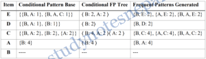
Hence, the frequent patterns generated are: {B, E: 2}, {A, E: 2}, {B, A, E: 2}, {B, D: 2}, {B, C: 4}, {A, C: 4}, {B, A, C: 2} and {B, A: 4}
The FP-growth method transforms the problem of finding long frequent patterns to searching for shorter ones recursively and then concatenating the suffix. It uses the least frequent items as a suffix, offering good selectivity. The method substantially reduces the search costs.
Handling Categorical Attributes
There are many applications that contain symmetric binary and nominal attributes. The Internet survey data shown in Table 3 contains symmetric binary attributes such as Gender, Computer at Home, Chat Online, Shop Online, and Privacy Concerns; as well as nominal attributes such as Level of Education and State. Using association analysis, we may uncover interesting information about the characteristics of Internet users such as:
{Shop Online = Yes} → {Privacy Concerns = Yes}
This rule suggests that most Internet users who shop online are concerned about their personal privacy.

To extract such patterns, the categorical and symmetric binary attributes are transformed into “items” first, so that existing association rule mining algorithms can be applied. This type of transformation can be performed by creating a new item for each distinct attribute-value pair. For example, the nominal attribute Level of Education can be replaced by three binary items: Education = College, Education = Graduate, and Education = High School. Similarly, symmetric binary attributes such as Gender can be converted into a pair of binary items, MaIe and Female. Table 4 shows the result of binarizing the Internet survey data

There are several issues to consider when applying association analysis to the binarized data:
Some attribute values may not be frequent enough to be part of a frequent pattern. This problem is more evident for nominal attributes that have many possible values, e.g., state names. Lowering the support threshold does not help because it exponentially increases the number of frequent patterns found (many of which may be spurious) and makes the computation more expensive. A more practical solution is to group related attribute values into a small number of categories. For example, each state name can be replaced by its corresponding geographical region, such as Midwest, Pacific Northwest, Southwest, and East Coast. Another possibility is to aggregate the less frequent attribute values into a single category called “Others”.
Some attribute values may have considerably higher frequencies than others. For example, suppose 85% of the survey participants own a home computer. By creating a binary item for each attribute value that appears frequently in the data, we may potentially generate many redundant patterns.
References
[1] J. Han and K. Micheline, Data Mining: Concepts and Techniques, San Francisco: Elsevier Inc., 2006.
[2] P.N. Tan, M. Steinbach and V. Kumar, INTRODUCTION TO DATA MINING, New York: PEARSON Addison Wesley, 2006.
[3] I. H. Witten and E. Frank, Data Mining Practical Machine Learning Tools and Techniques, San Francisco: Morgan Kaufmann Publishers, 2005.